K-means Clustering
In this this exercise, you will implement the K-means algorithm and use it for image compression.
- You will start with a sample dataset that will help you gain an intuition of how the K-means algorithm works.
- After that, you wil use the K-means algorithm for image compression by reducing the number of colors that occur in an image to only those that are most common in that image.
Outline
import numpy as np
import matplotlib.pyplot as plt
from utils import *

%matplotlib inline
1 - Implementing K-means
The K-means algorithm is a method to automatically cluster similar data points together.
Concretely, you are given a training set $\{x^{(1)}, ..., x^{(m)}\}$, and you want to group the data into a few cohesive “clusters”.
K-means is an iterative procedure that
- Starts by guessing the initial centroids, and then
- Refines this guess by
- Repeatedly assigning examples to their closest centroids, and then
- Recomputing the centroids based on the assignments.
In pseudocode, the K-means algorithm is as follows:
# Initialize centroids
# K is the number of clusters
centroids = kMeans_init_centroids(X, K)

for iter in range(iterations):
    # Cluster assignment step:
    # Assign each data point to the closest centroid.
    # idx[i] corresponds to the index of the centroid
    # assigned to example i
    idx = find_closest_centroids(X, centroids)

    # Move centroid step:
    # Compute means based on centroid assignments
    centroids = compute_means(X, idx, K)
The inner-loop of the algorithm repeatedly carries out two steps:
- (i) Assigning each training example $x^{(i)}$ to its closest centroid, and
- (ii) Recomputing the mean of each centroid using the points assigned to it.
The $K$-means algorithm will always converge to some final set of means for the centroids.
However, that the converged solution may not always be ideal and depends on the initial setting of the centroids.
- Therefore, in practice the K-means algorithm is usually run a few times with different random initializations.
- One way to choose between these different solutions from different random initializations is to choose the one with the lowest cost function value (distortion).
You will implement the two phases of the K-means algorithm separately in the next sections.
- You will start by completing
find_closest_centroidand then proceed to completecompute_centroids.
1.1 Finding closest centroids
In the “cluster assignment” phase of the K-means algorithm, the algorithm assigns every training example $x^{(i)}$ to its closest centroid, given the current positions of centroids.
Exercise 1
Your task is to complete the code in find_closest_centroids.
- This function takes the data matrix
Xand the locations of all centroids insidecentroids - It should output a one-dimensional array
idx(which has the same number of elements asX) that holds the index of the closest centroid (a value in $\{1,...,K\}$, where $K$ is total number of centroids) to every training example . - Specifically, for every example $x^{(i)}$ we set $$c^{(i)} := j \quad \mathrm{that \; minimizes} \quad ||x^{(i)} - \mu_j||^2,$$ where
- $c^{(i)}$ is the index of the centroid that is closest to $x^{(i)}$ (corresponds to
idx[i]in the starter code), and - $\mu_j$ is the position (value) of the $j$’th centroid. (stored in
centroidsin the starter code)
If you get stuck, you can check out the hints presented after the cell below to help you with the implementation.
# UNQ_C1
# GRADED FUNCTION: find_closest_centroids

def find_closest_centroids(X, centroids):
    """
    Computes the centroid memberships for every example

    Args:
        X (ndarray): (m, n) Input values
        centroids (ndarray): k centroids

    Returns:
        idx (array_like): (m,) closest centroids

    """

    # Set K
    K = centroids.shape[0]

    # You need to return the following variables correctly
    idx = np.zeros(X.shape[0], dtype=int)

    ### START CODE HERE ###

    ### END CODE HERE ###

    return idx
Click for hints
Here's how you can structure the overall implementation for this function
def find_closest_centroids(X, centroids):

    # Set K
    K = centroids.shape[0]

    # You need to return the following variables correctly
    idx = np.zeros(X.shape[0], dtype=int)

    ### START CODE HERE ###
    for i in range(X.shape[0]):
        # Array to hold distance between X[i] and each centroids[j]
        distance = []
        for j in range(centroids.shape[0]):
            norm_ij = # Your code to calculate the norm between (X[i] - centroids[j])
            distance.append(norm_ij)

        idx[i] = # Your code here to calculate index of minimum value in distance
    ### END CODE HERE ###
    return idx
If you're still stuck, you can check the hints presented below to figure out how to calculate
norm_ijandidx[i].Hint to calculate norm_ij
You can use np.linalg.norm to calculate the normMore hints to calculate norm_ij
You can compute norm_ij asnorm_ij = np.linalg.norm(X[i] - centroids[j])Hint to calculate idx[i]
You can use np.argmin to find the index of the minimum valueMore hints to calculate idx[i]
You can compute idx[i] asidx[i] = np.argmin(distance)
Now let's check your implementation using an example dataset
# Load an example dataset that we will be using
X = load_data()
The code below prints the first five elements in the variable X and the dimensions of the variable
print("First five elements of X are:\n", X[:5])
print('The shape of X is:', X.shape)
# Select an initial set of centroids (3 Centroids)
initial_centroids = np.array([[3,3], [6,2], [8,5]])

# Find closest centroids using initial_centroids
idx = find_closest_centroids(X, initial_centroids)

# Print closest centroids for the first three elements
print("First three elements in idx are:", idx[:3])

# UNIT TEST
from public_tests import *

find_closest_centroids_test(find_closest_centroids)
Expected Output:
| First three elements in idx are | [0 2 1] |
1.2 Computing centroid means
Given assignments of every point to a centroid, the second phase of the algorithm recomputes, for each centroid, the mean of the points that were assigned to it.
Exercise 2
Please complete the compute_centroids below to recompute the value for each centroid
Specifically, for every centroid $\mu_k$ we set $$\mu_k = \frac{1}{|C_k|} \sum_{i \in C_k} x^{(i)}$$
where
- $C_k$ is the set of examples that are assigned to centroid $k$
- $|C_k|$ is the number of examples in the set $C_k$
Concretely, if two examples say $x^{(3)}$ and $x^{(5)}$ are assigned to centroid $k=2$, then you should update $\mu_2 = \frac{1}{2}(x^{(3)}+x^{(5)})$.
If you get stuck, you can check out the hints presented after the cell below to help you with the implementation.
# UNQ_C2
# GRADED FUNCTION: compute_centpods

def compute_centroids(X, idx, K):
    """
    Returns the new centroids by computing the means of the
    data points assigned to each centroid.

    Args:
        X (ndarray):   (m, n) Data points
        idx (ndarray): (m,) Array containing index of closest centroid for each
                       example in X. Concretely, idx[i] contains the index of
                       the centroid closest to example i
        K (int):       number of centroids

    Returns:
        centroids (ndarray): (K, n) New centroids computed
    """

    # Useful variables
    m, n = X.shape

    # You need to return the following variables correctly
    centroids = np.zeros((K, n))

    ### START CODE HERE ###

    ### END CODE HERE ##

    return centroids
Click for hints
Here's how you can structure the overall implementation for this function
def compute_centroids(X, idx, K):
    # Useful variables
    m, n = X.shape

    # You need to return the following variables correctly
    centroids = np.zeros((K, n))

    ### START CODE HERE ###
    for k in range(K):
        points = # Your code here to get a list of all data points in X assigned to centroid k
        centroids[k] = # Your code here to compute the mean of the points assigned
### END CODE HERE ##

return centroids
If you're still stuck, you can check the hints presented below to figure out how to calculate
pointsandcentroids[k].Hint to calculate points
Say we wanted to find all the values in X that were assigned to clusterk=0. That is, the corresponding value in idx for these examples is 0. In Python, we can do it asX[idx == 0]. Similarly, the points assigned to centroidk=1areX[idx == 1]More hints to calculate points
You can compute points aspoints = X[idx == k]Hint to calculate centroids[k]
You can use np.mean to find the mean. Make sure to set the parameteraxis=0More hints to calculate centroids[k]
You can compute centroids[k] ascentroids[k] = np.mean(points, axis = 0)
Now check your implementation by running the cell below
K = 3
centroids = compute_centroids(X, idx, K)

print("The centroids are:", centroids)

# UNIT TEST
compute_centroids_test(compute_centroids)
Expected Output:
2.42830111 3.15792418
5.81350331 2.63365645
7.11938687 3.6166844
2 - K-means on a sample dataset
After you have completed the two functions (find_closest_centroids
and compute_centroids) above, the next step is to run the
K-means algorithm on a toy 2D dataset to help you understand how
K-means works.
- We encourage you to take a look at the function (
run_kMeans) below to understand how it works. - Notice that the code calls the two functions you implemented in a loop.
When you run the code below, it will produce a visualization that steps through the progress of the algorithm at each iteration.
- At the end, your figure should look like the one displayed in Figure 1.
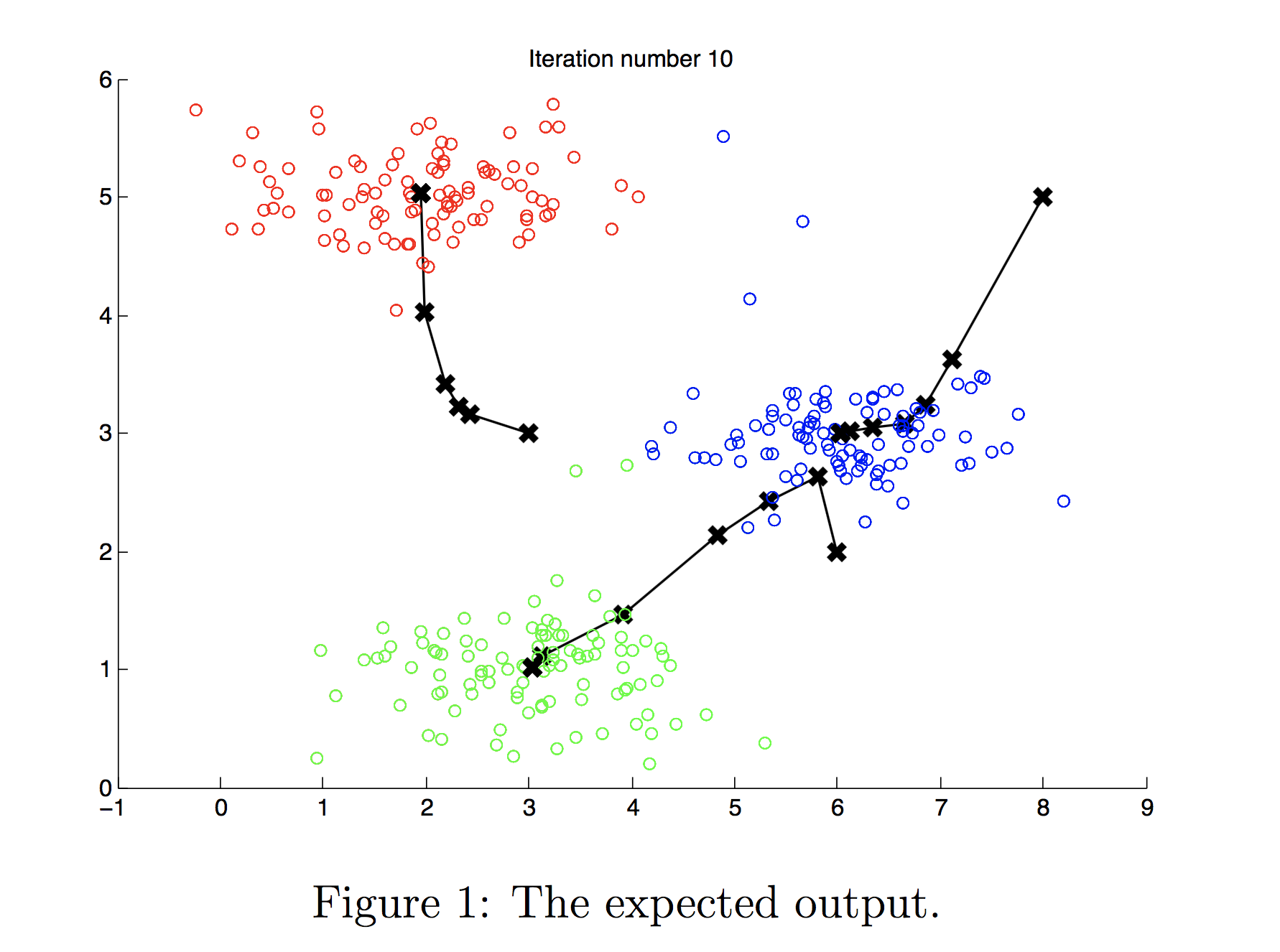
Note: You do not need to implement anything for this part. Simply run the code provided below
# You do not need to implement anything for this part

def run_kMeans(X, initial_centroids, max_iters=10, plot_progress=False):
    """
    Runs the K-Means algorithm on data matrix X, where each row of X
    is a single example
    """

    # Initialize values
    m, n = X.shape
    K = initial_centroids.shape[0]
    centroids = initial_centroids
    previous_centroids = centroids
    idx = np.zeros(m)

    # Run K-Means
    for i in range(max_iters):

        #Output progress
        print("K-Means iteration %d/%d" % (i, max_iters-1))

        # For each example in X, assign it to the closest centroid
        idx = find_closest_centroids(X, centroids)

        # Optionally plot progress
        if plot_progress:
            plot_progress_kMeans(X, centroids, previous_centroids, idx, K, i)
            previous_centroids = centroids

        # Given the memberships, compute new centroids
        centroids = compute_centroids(X, idx, K)
    plt.show()
    return centroids, idx
# Load an example dataset
X = load_data()

# Set initial centroids
initial_centroids = np.array([[3,3],[6,2],[8,5]])
K = 3

# Number of iterations
max_iters = 10

centroids, idx = run_kMeans(X, initial_centroids, max_iters, plot_progress=True)
3 - Random initialization
The initial assignments of centroids for the example dataset was designed so that you will see the same figure as in Figure 1. In practice, a good strategy for initializing the centroids is to select random examples from the training set.
In this part of the exercise, you should understand how the function kMeans_init_centroids is implemented.
- The code first randomly shuffles the indices of the examples (using
np.random.permutation()). - Then, it selects the first $K$ examples based on the random permutation of the indices.
- This allows the examples to be selected at random without the risk of selecting the same example twice.
Note: You do not need to make implement anything for this part of the exercise.
# You do not need to modify this part

def kMeans_init_centroids(X, K):
    """
    This function initializes K centroids that are to be
    used in K-Means on the dataset X

    Args:
        X (ndarray): Data points
        K (int):     number of centroids/clusters

    Returns:
        centroids (ndarray): Initialized centroids
    """

    # Randomly reorder the indices of examples
    randidx = np.random.permutation(X.shape[0])

    # Take the first K examples as centroids
    centroids = X[randidx[:K]]

    return centroids
4 - Image compression with K-means
In this exercise, you will apply K-means to image compression.
- In a straightforward 24-bit color representation of an image$^{2}$, each pixel is represented as three 8-bit unsigned integers (ranging from 0 to 255) that specify the red, green and blue intensity values. This encoding is often refered to as the RGB encoding.
- Our image contains thousands of colors, and in this part of the exercise, you will reduce the number of
In this part, you will use the K-means algorithm to select the 16 colors that will be used to represent the compressed image.
- Concretely, you will treat every pixel in the original image as a data example and use the K-means algorithm to find the 16 colors that best group (cluster) the pixels in the 3- dimensional RGB space.
- Once you have computed the cluster centroids on the image, you will then use the 16 colors to replace the pixels in the original image.
$^{2}$The provided photo used in this exercise belongs to Frank Wouters and is used with his permission.
4.1 Dataset
Load image
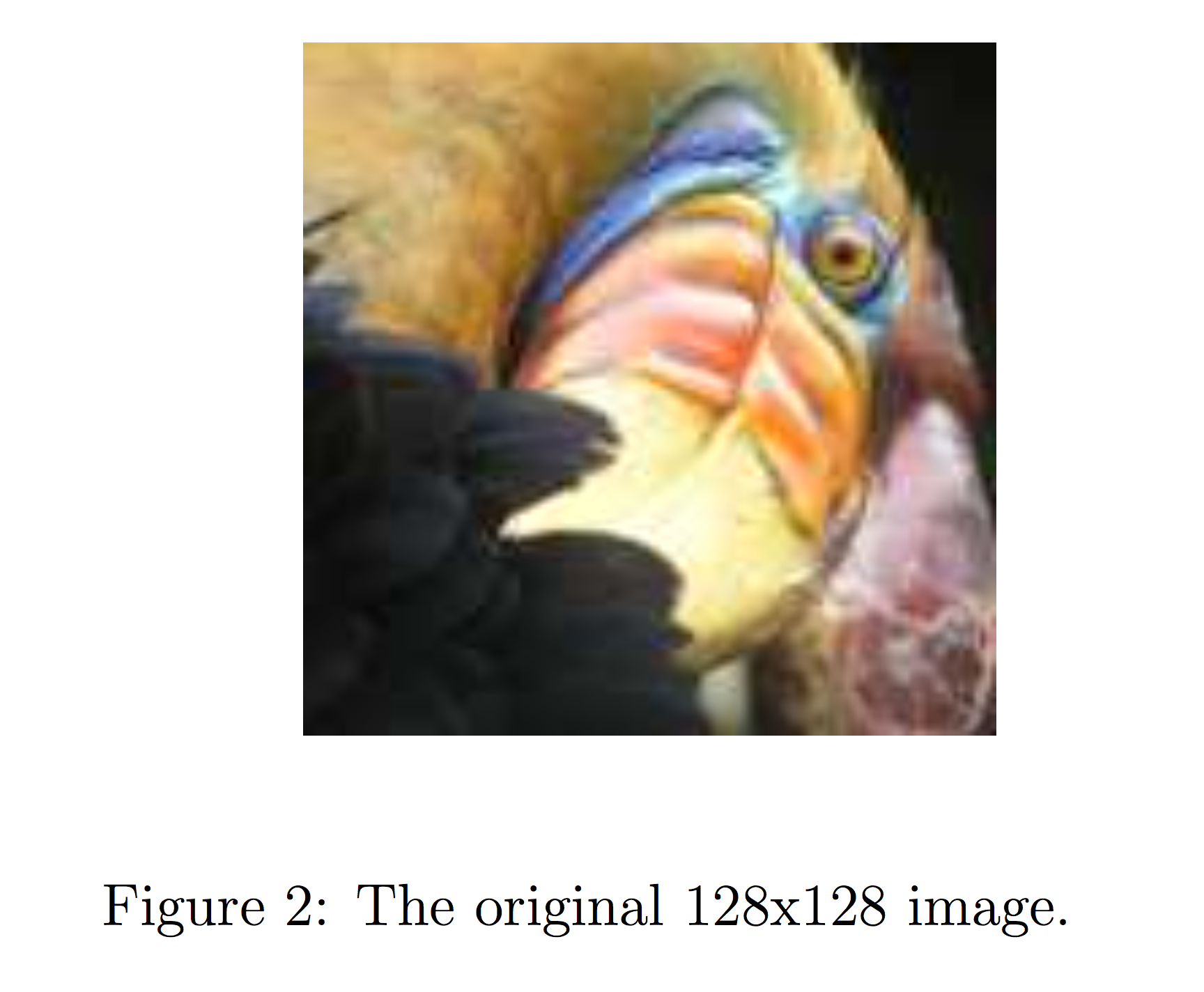
First, you will use matplotlib to read in the original image, as shown below.
# Load an image of a bird
original_img = plt.imread('bird_small.png')
Visualize image
You can visualize the image that was just loaded using the code below.
# Visualizing the image
plt.imshow(original_img)
Check the dimension of the variable
As always, you will print out the shape of your variable to get more familiar with the data.
print("Shape of original_img is:", original_img.shape)
As you can see, this creates a three-dimensional matrix original_img where
- the first two indices identify a pixel position, and
- the third index represents red, green, or blue.
For example, original_img[50, 33, 2] gives the blue intensity of the pixel at row 50 and column 33.
Processing data
To call the run_kMeans, you need to first transform the matrix original_img into a two-dimensional matrix.
- The code below reshapes the matrix
original_imgto create an $m \times 3$ matrix of pixel colors (where $m=16384 = 128\times128$)
# Divide by 255 so that all values are in the range 0 - 1
original_img = original_img / 255

# Reshape the image into an m x 3 matrix where m = number of pixels
# (in this case m = 128 x 128 = 16384)
# Each row will contain the Red, Green and Blue pixel values
# This gives us our dataset matrix X_img that we will use K-Means on.

X_img = np.reshape(original_img, (original_img.shape[0] * original_img.shape[1], 3))
# Run your K-Means algorithm on this data
# You should try different values of K and max_iters here
K = 16
max_iters = 10

# Using the function you have implemented above.
initial_centroids = kMeans_init_centroids(X_img, K)

# Run K-Means - this takes a couple of minutes
centroids, idx = run_kMeans(X_img, initial_centroids, max_iters)
print("Shape of idx:", idx.shape)
print("Closest centroid for the first five elements:", idx[:5])
4.3 Compress the image
After finding the top $K=16$ colors to represent the image, you can now
assign each pixel position to its closest centroid using the
find_closest_centroids function.
- This allows you to represent the original image using the centroid assignments of each pixel.
- Notice that you have significantly reduced the number of bits that are required to describe the image.
- The original image required 24 bits for each one of the $128\times128$ pixel locations, resulting in total size of $128 \times 128 \times 24 = 393,216$ bits.
- The new representation requires some overhead storage in form of a dictionary of 16 colors, each of which require 24 bits, but the image itself then only requires 4 bits per pixel location.
- The final number of bits used is therefore $16 \times 24 + 128 \times 128 \times 4 = 65,920$ bits, which corresponds to compressing the original image by about a factor of 6.
# Represent image in terms of indices
X_recovered = centroids[idx, :]

# Reshape recovered image into proper dimensions
X_recovered = np.reshape(X_recovered, original_img.shape)
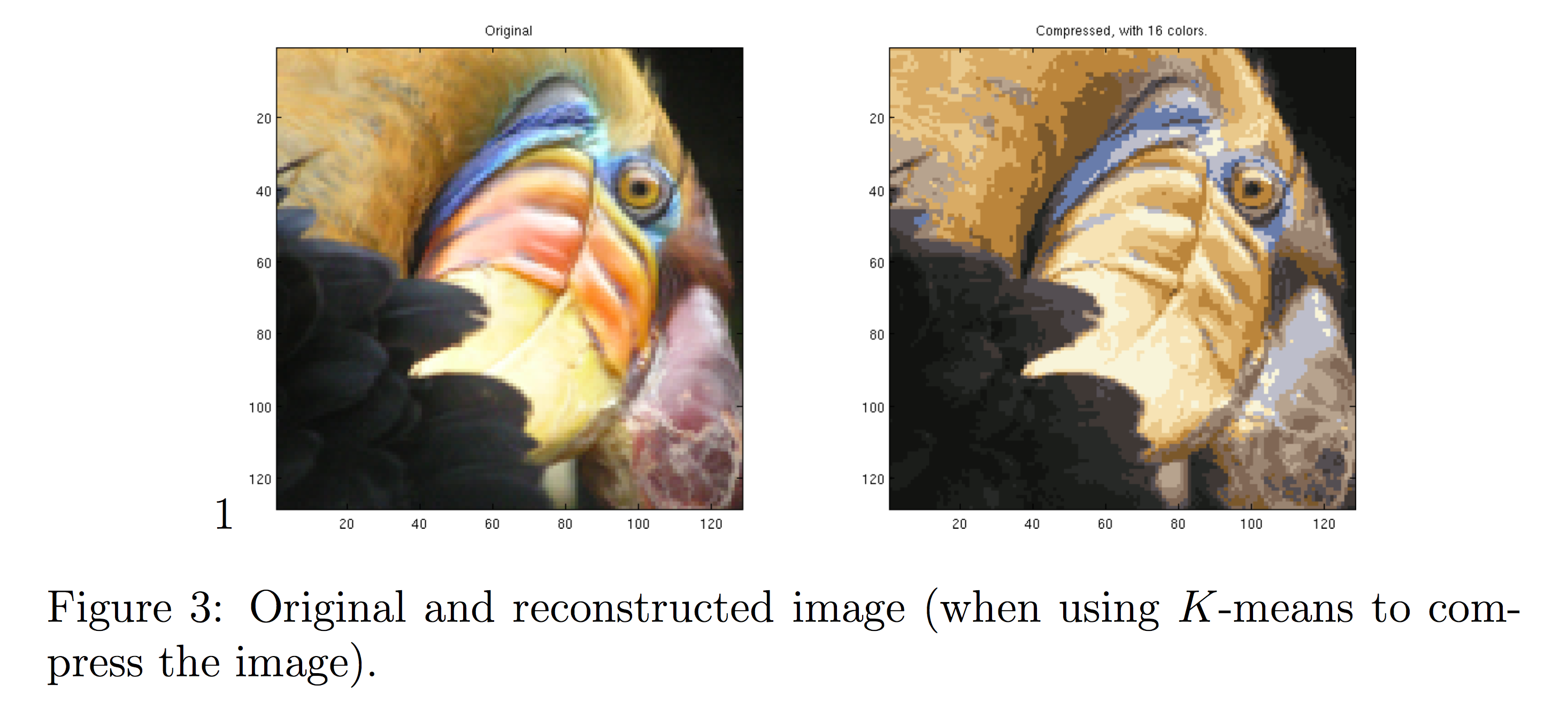
Finally, you can view the effects of the compression by reconstructing the image based only on the centroid assignments.
- Specifically, you can replace each pixel location with the mean of the centroid assigned to it.
- Figure 3 shows the reconstruction we obtained. Even though the resulting image retains most of the characteristics of the original, we also see some compression artifacts.
# Display original image
fig, ax = plt.subplots(1,2, figsize=(8,8))
plt.axis('off')

ax[0].imshow(original_img*255)
ax[0].set_title('Original')
ax[0].set_axis_off()


# Display compressed image
ax[1].imshow(X_recovered*255)
ax[1].set_title('Compressed with %d colours'%K)
ax[1].set_axis_off()